Transformers and Perfomers
Review the attention mechanism and performers
Recently, there has been a new surge in machine learning community studying attention mechanism in transformers in both theory and practice. The concept attention here is proposed by authors from Google
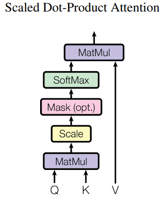
Attention
Given an input $X$, we consider a triplet $(K, Q, V)$ which is the results of three linear transformations. Each component in this triplet is coined as
- $K$: key
- $Q$: query
- $V$: value
This formula can be intuitively understood as we want an output which is a weighted sum of values. The weight here is decided by how compatible between the query and the key it is.
Indeed the term “attention” is come from the computed weight. The more weight is assigned, the more attention is put on a feature dimension of value $V$. There is no outside knowledge involved except the input $X$.

This is the basic building block of surprisingly successful models such as GPT-2, GPT-3 which are composed of concatenations of attentions as well as multilayers of attentions. This post will not discuss further the architures of these models, but move on to an extension of attentions in which we can further reduce computational cost of this type of operators.
Performers
The main focus of Perfomer is to address the issue of the attention mechanism which scales quadratically w.r.t. the number of tokens. Note that the input of transformers usually a sequence of tokens. Such a computation cost may not be allowed when data contains long sequences.
The Performer paper
Here, $D^{-1}A$ is just another way to represent $softmax(\cdot)$. $A$ stands for the attention matrix.
Kernelizable attention The paper explains that we can express the attention matrix as a kernel
\[A(i,j) = K(q_i, k_j)\]We expect to approximate the kernel with a new representation
\[K(x,y) = \mathbb{E}[\phi(x)^\top \phi(y)]\]Now the main question is how to makes this resprentation is cheaper to compute. Assume we already have such approximation, the approximated attention matrix now is (no longer has $\exp(\cdot)$ outside)
\[A = Q' K'^\top, \quad Q', K' \in \mathbb{R}^{L\times r}\]A bit of literature review Kernel approximation has a quite history. One of the notable work is random Fourier feature (RFF)
The goal is to find a feature map $\phi(\cdot)$ such that $K(x, y) = \mathbb{E}_\omega [\phi(x)^\top \phi(y)]$. Simply by rearranging the last term in Bochner’s theorem, we can have something similar to dot-product and the integral is approximated and Monte Carlo integration. The random Fourier feature maps are in the form of sine and/or cosine transformation of linear transformation of inputs. The linear weights are sampled from spectral density.
In Gaussian Process research, Spectral Mixture kernel is originated from the same idea where we need to design the spectral distribution to obtain new types of kernels
What is the approximate feature map for attention?
The Performer paper
where
- $w_i$ are sampled from a distribution $\mathcal{D}$
- $f_l$ are some functions
From the softmax kernel, we have \(\begin{aligned} SM(x, y) = & \exp(x^\top y) = \exp\left(-\frac{\lVert x - y \rVert^2}{2} + \frac{\lVert x \rVert^2}{2}+ \frac{\lVert y \rVert^2}{2}\right)\\ = &\exp\left(\frac{\lVert x \rVert^2}{2}\right) K_{\text{Gaussian}}(x, y)\exp\left(\frac{\lVert y \rVert^2}{2}\right) \end{aligned}\)
Obviously, RFF provides us the approximation for $K_{\text{Gaussian}}$ so we can easily derive the feature map.
However, the paper discusses a numerical problem that computing the renomalized $D^{-1}$ may encounter negative values due to sampling procedure. To avoid this, the paper suggests two options of choosing feature map:
- Case 1: $h(x)=\exp(-\lVert x \rVert^2/2 ), l=1, f_1 = \exp, \mathcal{D} = \mathcal{N}(0, I)$
- Case 2: $h(x)=\frac{1}{\sqrt{2}}\exp(-\lVert x \rVert^2/2 ), l=2, f_1(u) = \exp(u),f_2(u) = \exp(-u), \mathcal{D} = \mathcal{N}(0, I)$
The paper further provided the convergence analysis for such approximations including showing unbiased estimation and variance reduction.
Computational benefit
The main difference between the computational cost of the original attension and those of the performer is that we use $Q^{\prime}{K^{\prime}}^\top$ instead of $\exp(QK^\top)$. However, to realize the real computational cost, we may need to rearrange the parenthesis
\[Attention(Q, K, V) \approx \hat{D}^{-1} (Q'K'^\top) V = \hat{D}^{-1} (Q'(K'^\top V)).\]Let’s say $Q, K \in \mathbb{R}^{L\times d}$ and $Q^{\prime}, K^{\prime} \in \mathbb{R}^{L\times m}, m < d$. So the computational cost is $\mathcal{O}(Lm + Ld + md)$ which is better than quadratic w.r.t $L$.