From Neural ODEs to Neural SDEs
Understanding the method solving neural stochastic differential equations
When writing this series of stochastic calculus, there has been a much development among machine learning community adopting stochastic differential equation in neural networks. It starts with Neural Ordinary Equations
The key techniques include adjoint sentitivity method in performing backpropagragtion through time (not layers), and quering sample paths from forward-pass when solving backward SDEs. This post focuses more on the former, and just briefly mention the latter.
Neural ODEs
Neural Ordinary Differential Equations (Neural ODEs) are inspired by a model construction like residual networks, recurrent neural network, and based on the following generalization
By doing so, the discrete layer index in neural network is now understood as continous time index in dynamic systems modeled by an ODE.
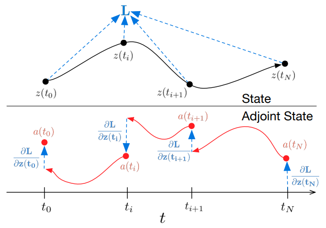
Adjoint sentivity method for backpropagation In learning neural network, given an input, we need to forward it by feed to model to produce output. The goal is to compute a gradient w.r.t. $\theta$ so that the parameters will be optimized by gradient descent methods. Computing such a gradient is known as backpropagation, running backward from output through very layer. If there is no discrete layer, how do we backpropagate here?
In fact, in neural ODEs, at the forward-pass, the output is obtained via a ODE solver which does discretize continuous into smaller time steps. Therefore, we can backpropagate via these intermediate steps. However, it is required to store all of information of these steps to perform normal backward-pass. Avoiding this is one of main contribution of neural ODE.
Formally, we want to compute the gradient $dL/d\theta$ of
\[L(z(t_1)) = L\left(z(t_0) + \int_{t_0}^{t_1} f(z(t); \theta) dt\right) = L(\texttt{ODESolve}(z(t_0), f, t_0, t_1; \theta))\]where $L(\cdot)$ is a loss function.
The adjoint sensitivity method compute $dL/d\theta$ with an extra helping hand of a new guy called adjoint $a(t) = \partial L / \partial z(t)$ which agrees with a ODE (red texts use 1-chain rule, 2-Taylor expansion)
\[\begin{aligned} \frac{da(t)}{dt} = & \lim_{\varepsilon \to 0} \frac{a(t + \varepsilon) - a(t)}{\varepsilon} \\ = & \lim_{\varepsilon \to 0} \frac{a(t + \varepsilon) - \textcolor{red}{\frac{dL}{dz(t)}}}{\varepsilon}\\ = & \lim_{\varepsilon \to 0} \frac{a(t + \varepsilon) - \textcolor{red}{\frac{dL}{dz(t + \varepsilon)} \frac{dz(t + \varepsilon)}{dz(t)} }}{\varepsilon}\\ = & \lim_{\varepsilon \to 0} \frac{a(t + \varepsilon) - \textcolor{red}{a(t+\varepsilon) (I + \varepsilon f(z(t)) + \mathcal{O}(\varepsilon^2))}}{\varepsilon}\\ = & - a(t)^\top \frac{\partial f(z(t), t, \theta)}{\partial z} \end{aligned}\]We then need to solve this new ODE to obtain the gradient w.r.t. $\theta$:
\[\frac{dL}{d\theta} = - \int_{t_1}^{t_0} a(t)^\top \frac{\partial f(z(t), t, \theta)}{\partial \theta} dt\]So, this is the main technical background of Neural ODE.

Neural SDEs
With the same motivation, neural stochastic differential equations (Neural SDEs) is extended from Neural ODEs where randomness is injected to equations.
Consider the following SDEs
\[dZ_t = \mu(t, Z_t) dt + \sigma(t, Z_t) \circ dW_t\]where $\circ$ indicates Stratonovich-style stochastic integral.
Adjoint sensitivity with noise Similar to Neural ODEs, we define adjoint term as $A_t = dL(Z_T)/dZ_t$ which is now a stochastic process satisfying
\[dA_t^i = - A_t^j \frac{\partial \mu^j}{\partial Z^i}(t, Z_t) dt - \frac{\partial \sigma^{i,k}}{\partial Z^i}(t, Z_t) \circ dW^k_t\]Here, we have to solve this new SDE backward from $t=T$ to $t=0$ conditioning on $A_T = dL(Z_T)/dZ_T$ where $Z_T$ is obtained from the forward-pass.
Challenge in solving backward SDE The main different with Neural ODEs lies in the stochastic part. The sample path of Browian motion to compute $Z_T$ in the forward-pass needs to be retrieved during backward-pass.
Current related ML research
Here are some hightlights of related research:
- Deep limits
: Providing a contruction from discrete to continuous. However, diffusion function is considered as a constant. - Learning Neural SDEs with adversarial approach
. - Uncertanty estimation for neural networks
where the drift function (modeled by a neural network) is to make prediction and the diffusion function is to measure the uncertainty. - Application in Finance
.
Closing thought
Many applications relying on SDEs often use a simple form of drift function $\mu$ and diffusion function $\sigma$. Now with the new approach in ML, we have a better tool to work with higher dimension of these functions as well as more expressive forms with more parameters. The strength of ML approach is that it can provide a nice estimations for such hyperparameters.